Kaggle竞赛——房价预测

1. 特征分析
- 1.1 数据集导入
- 1.2 统计缺失值
- 1.3 可视化缺失值
- 1.4 缺失值相关性分析
- 1.5 训练集和测试集缺失数据对比
- 1.6 统计特征的数据类型
- 1.7 数值型特征分布直方图
- 1.8 数值型特征与房价的线性关系
- 1.9 非数值型特征的分布直方图
- 1.10 非数值型特征箱线图
- 1.11 数值型特征填充前后的分布对比
- 1.12 时序特征分析
- 1.13 用热图分析数值型特征之间的相关性
2. 数据处理
- 2.1 正态化 SalePrice
- 2.2 时序特征处理
- 2.3 特征融合
- 2.4 填充特征值
- 2.5 连续性数据正态化
- 2.5 编码数据集后切分数据集
3. 模型搭建
- 3.1 模型搭建与超参数调整
- 3.2 模型交叉验证
- 3.3 特征重要性分析
- 3.4 数值预测
4. 参考文献

这是接触Kaggle竞赛的第一个题目，借鉴了其他人可视化分析和特征分析的技巧（文末附链接）。本次提交到Kaggle的得分是0.13227，排名1209（提交日期：2024年6月30日），数据集和代码已经打包放到Gitee，点击直达。
在这里插入图片描述
思路简图：

1. 特征分析

1.1 数据集导入

将训练集与测试集合并，方便更准确地分析数据特征。

train = pd.read_csv("D:\\Desktop\\kaggle数据集\\house-prices-advanced-regression-techniques\\train.csv")
test  = pd.read_csv("D:\\Desktop\\kaggle数据集\\house-prices-advanced-regression-techniques\\test.csv")
Id = test['Id']
print("训练集大小{}".format(train.shape))
print("测试集大小{}".format(test.shape))
# 合并训练集与测试集，方便更准确地分析数据特征
datas = pd.concat([train, test], ignore_index=True)
# 删除Id列
datas.drop("Id", axis= 1, inplace=True)

训练集大小(1460, 81)
测试集大小(1459, 80)

1.2 统计缺失值

#------------------------------------------------------------------------------------------------------------#
# 统计数据集中的值的空缺情况（以列为统计单位）
# isnull()：检查所有数据集，如果是缺失值则返回True，否则返回False
# .sum()：计算每列中True的数量
#------------------------------------------------------------------------------------------------------------#
datas.isnull().sum().sort_values(ascending = False).head(40)

PoolQC           2909
MiscFeature      2814
Alley            2721
Fence            2348
MasVnrType       1766
SalePrice        1459
FireplaceQu      1420
LotFrontage       486
GarageFinish      159
GarageQual        159
GarageCond        159
GarageYrBlt       159
GarageType        157
BsmtCond           82
BsmtExposure       82
BsmtQual           81
BsmtFinType2       80
BsmtFinType1       79
MasVnrArea         23
MSZoning            4
BsmtHalfBath        2
Utilities           2
BsmtFullBath        2
Functional          2
Exterior2nd         1
Exterior1st         1
GarageArea          1
GarageCars          1
SaleType            1
KitchenQual         1
BsmtFinSF1          1
Electrical          1
BsmtFinSF2          1
BsmtUnfSF           1
TotalBsmtSF         1
TotRmsAbvGrd        0
Fireplaces          0
SaleCondition       0
PavedDrive          0
MoSold              0
dtype: int64

1.3 可视化缺失值

右侧的微线图概括了数据完整性的一般形状，并标明了具有最多空值（最靠近左侧，数值表示的该行中非空值的数量）和最少空值（最靠近右侧）的行。

msno.matrix(datas)

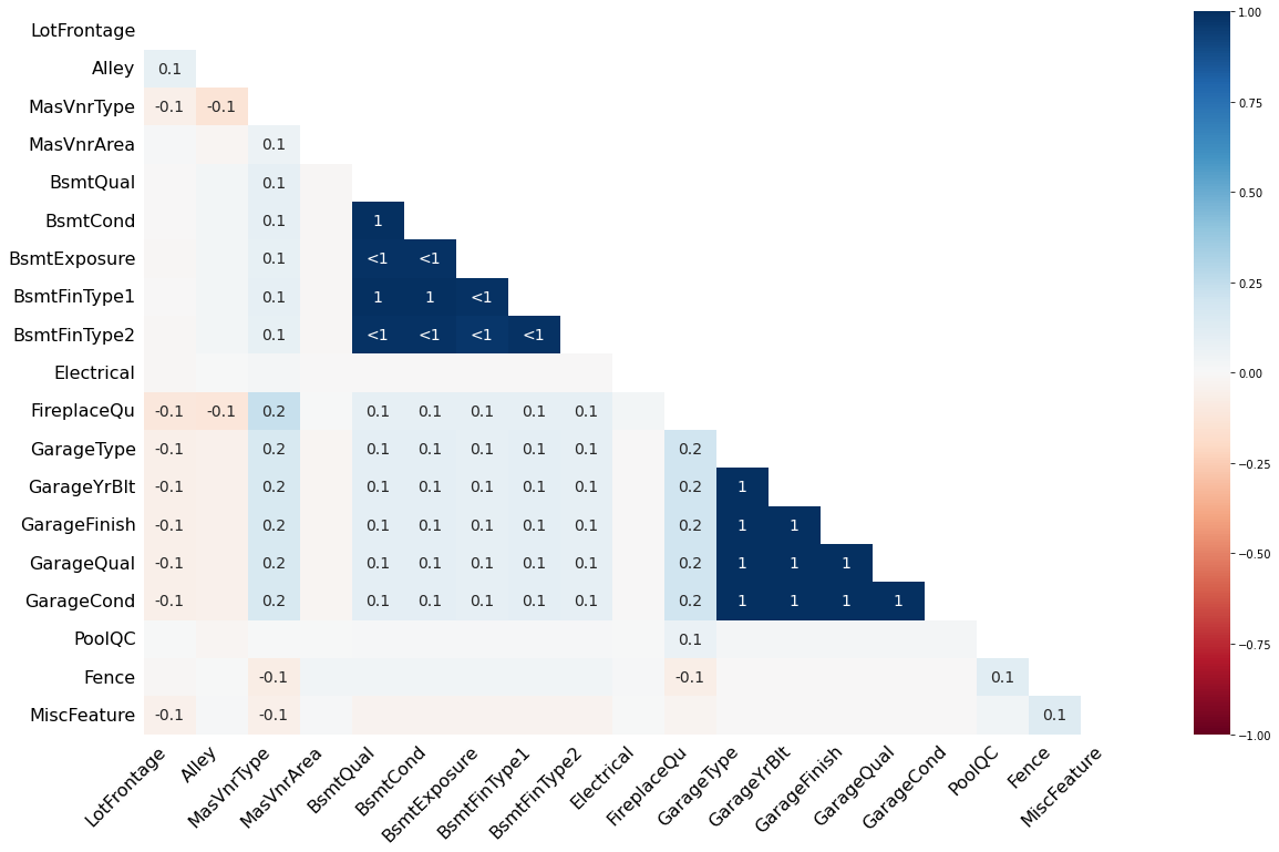
1.4 缺失值相关性分析

用热图显示数据集中缺失值之间的相关性

1：表示两个特征的缺失模式完全相同，即其中一个缺失时，另一个也缺失
-1：表示一个特征有缺失值时，另一个特征没有缺失值
0：表示两个特征的缺失值模式不相关

msno.heatmap(train)

在这里插入图片描述

1.5 训练集和测试集缺失数据对比

#------------------------------------------------------------------------------------------------------------#
# 比较两个dataframe（train和test）的数据类型，需确保两个数据集具有相同的列标签
#------------------------------------------------------------------------------------------------------------#
train_dtype = train_dtype.drop('SalePrice')
train_dtype.compare(test_dtype)

在这里插入图片描述
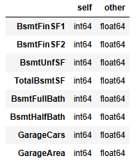
由对比结果可知数据类型都是int64和float64的区别，对结果影响不大。

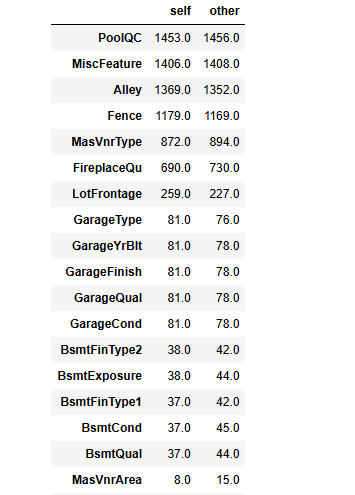
# 缺失值对比
null_train = train.isnull().sum()
null_test = test.isnull().sum()
null_train = null_train.drop('SalePrice')
null_comp = null_train.compare(null_test).sort_values(['self'], ascending=[False])
null_comp

（局部，未截完整）
在这里插入图片描述

1.6 统计特征的数据类型

数值型特征
- 1.1 离散特征（唯一值（多个重复值只取一个）数量小于25（可视情况而定））
- 1.2 连续特征（‘Id’列不计入）
非数值型数据

# 在 pandas 中,如果一个列的数据类型无法确定为数值型,则会被标记为 '0'
numerical_features = [col for col in datas.columns if datas[col].dtypes != 'O']
discrete_features = [col for col in numerical_features if len(datas[col].unique()) < 25]
continuous_features = [feature for feature in numerical_features if feature not in discrete_features]
non_numerical_features = [col for col in datas.columns if datas[col].dtype == 'O']

print("Total Number of Numerical Columns : ",len(numerical_features))
print("Number of discrete features : ",len(discrete_features))
print("No of continuous features are : ", len(continuous_features))
print("Number of non-numeric features : ",len(non_numerical_features))

print("离散型数据: ",discrete_features)
print("连续型数据：", continuous_features)
print("非数值型数据：",non_numerical_features)

Total Number of Numerical Columns :  37
Number of discrete features :  15
No of continuous features are :  22
Number of non-numeric features :  43
离散型数据:  ['MSSubClass', 'OverallQual', 'OverallCond', 'BsmtFullBath', 'BsmtHalfBath', 'FullBath', 'HalfBath', 'BedroomAbvGr', 'KitchenAbvGr', 'TotRmsAbvGrd', 'Fireplaces', 'GarageCars', 'PoolArea', 'MoSold', 'YrSold']
连续型数据： ['LotFrontage', 'LotArea', 'YearBuilt', 'YearRemodAdd', 'MasVnrArea', 'BsmtFinSF1', 'BsmtFinSF2', 'BsmtUnfSF', 'TotalBsmtSF', '1stFlrSF', '2ndFlrSF', 'LowQualFinSF', 'GrLivArea', 'GarageYrBlt', 'GarageArea', 'WoodDeckSF', 'OpenPorchSF', 'EnclosedPorch', '3SsnPorch', 'ScreenPorch', 'MiscVal', 'SalePrice']
非数值型数据： ['MSZoning', 'Street', 'Alley', 'LotShape', 'LandContour', 'Utilities', 'LotConfig', 'LandSlope', 'Neighborhood', 'Condition1', 'Condition2', 'BldgType', 'HouseStyle', 'RoofStyle', 'RoofMatl', 'Exterior1st', 'Exterior2nd', 'MasVnrType', 'ExterQual', 'ExterCond', 'Foundation', 'BsmtQual', 'BsmtCond', 'BsmtExposure', 'BsmtFinType1', 'BsmtFinType2', 'Heating', 'HeatingQC', 'CentralAir', 'Electrical', 'KitchenQual', 'Functional', 'FireplaceQu', 'GarageType', 'GarageFinish', 'GarageQual', 'GarageCond', 'PavedDrive', 'PoolQC', 'Fence', 'MiscFeature', 'SaleType', 'SaleCondition']

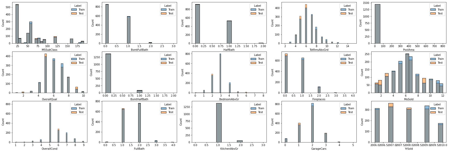
1.7 数值型特征分布直方图

离散数据分布直方图

#------------------------------------------------------------------------------------------------------------#
# 添加 Label 列用于标识训练集和测试集
#------------------------------------------------------------------------------------------------------------#
datas['Label'] = "Test"
datas['Label'][:1460] = "Train"

#------------------------------------------------------------------------------------------------------------#
# 离散数据直方图
# sharex=False：子图的x轴不共享，每个子图可以独立设置自己的x轴属性
# hue='Label'：根据 Label 列的值为直方图上色，不同的 Label 值会分配不同颜色
# ax=axes[i%3,i//3]：确保了直方图可以在一个3xN的网格中均匀分布
#------------------------------------------------------------------------------------------------------------#
fig, axes = plt.subplots(3, 5, figsize=(30, 10), sharex=False)
for i, feature in enumerate(discrete_features):
    sns.histplot(data=datas, x=feature, hue='Label', ax=axes[i%3, i//3])

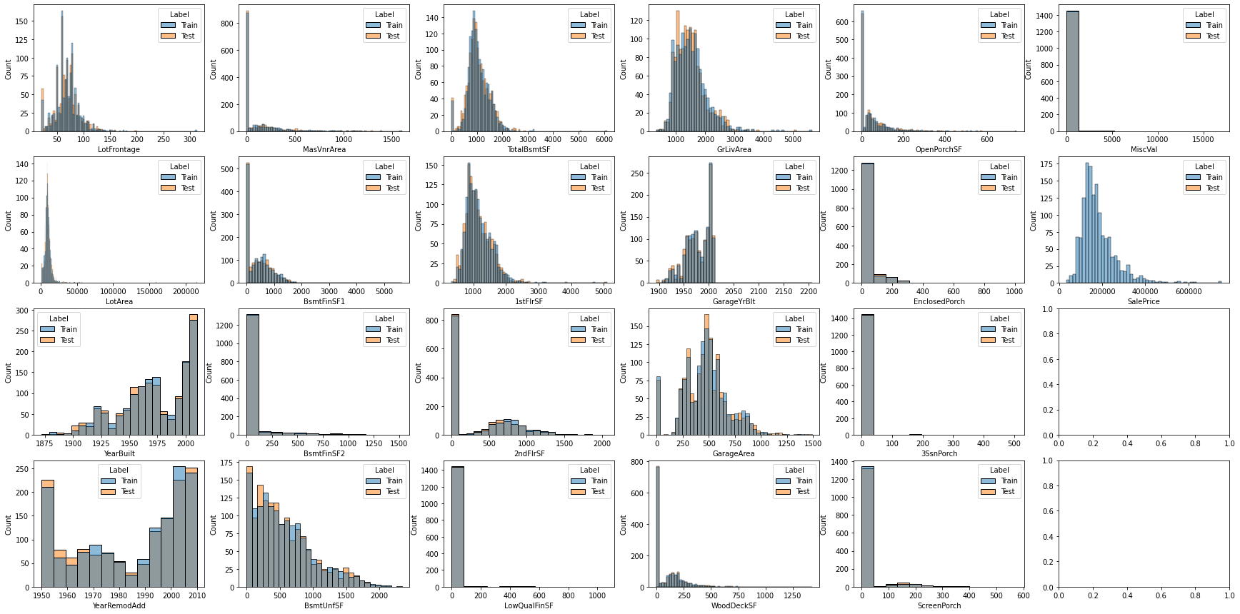
连续数据分布直方图

fig,axes = plt.subplots(nrows = 4, ncols = 6, figsize=(30,15), sharex=False)
for i, feature in enumerate(continuous_features):
    sns.histplot(data=datas, x=feature, hue='Label',ax=axes[i%4,i//4])

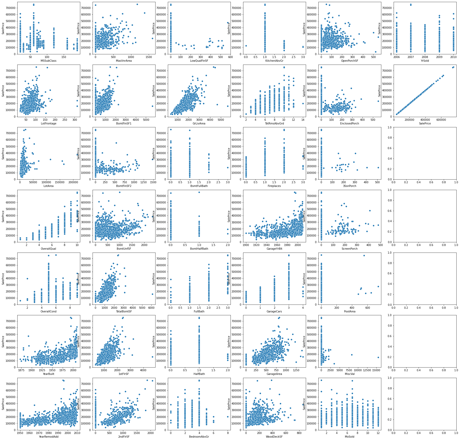
1.8 数值型特征与房价的线性关系

fig, axes = plt.subplots(7, 6, figsize=(30, 30), sharex=False)
for i, feature in enumerate(numerical_features):
    sns.scatterplot(data = datas, x = feature, y="SalePrice", ax=axes[i%7, i//7])

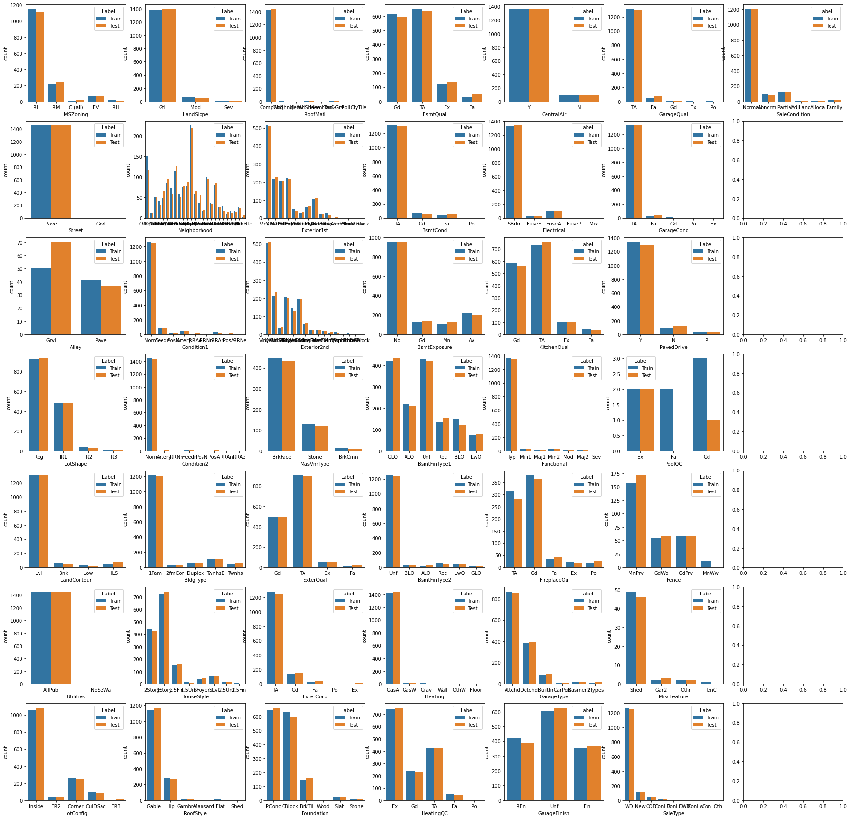
1.9 非数值型特征的分布直方图

f,axes = plt.subplots(7, 7, figsize=(30,30),sharex=False)
for i,feature in enumerate(non_numerical_features):
    sns.countplot(data=datas, x=feature, hue="Label", ax=axes[i%7,i//7])

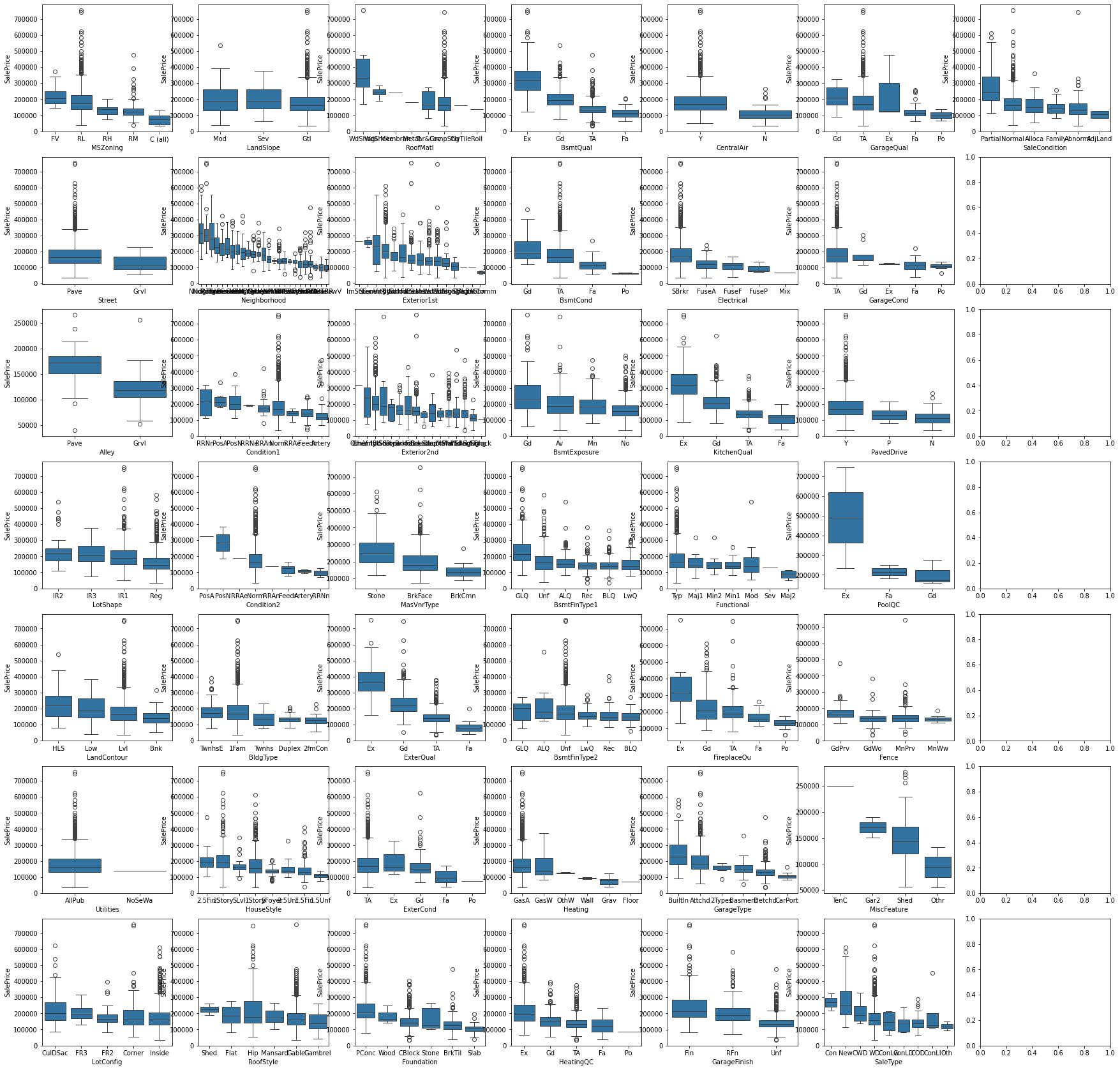
1.10 非数值型特征箱线图

对每个箱线图内部按照 SalePric 对不同的特征值进行降序排序。

#------------------------------------------------------------------------------------------------------------#
# groupby(feature)['SalePrice'].median()：计算每个 feature 分组的SalePrice中位数
# items()：将结果转换为一个包含键值对的迭代器（迭代器中的每个元素都是一个二元组），二元组形式：（特征值，中位数）
# x[1]：根据二元组的第二个值进行排序
# reverse = True：降序
# x[0] for x in sort_list：提取二元组的第一个值（键）即特征值
# order=order_list：按 order_list 中的顺序排列 x 轴的分类
#------------------------------------------------------------------------------------------------------------#
fig, axes = plt.subplots(7,7 , figsize=(30, 30), sharex=False)
for i, feature in enumerate(non_numerical_features):
    sort_list = sorted(datas.groupby(feature)['SalePrice'].median().items(), key = lambda x:x[1], reverse = True)
    order_list = [x[0] for x in sort_list ]
    sns.boxplot(data = datas, x = feature, y = 'SalePrice', order=order_list, ax=axes[i%7, i//7])
plt.show()

在这里插入图片描述

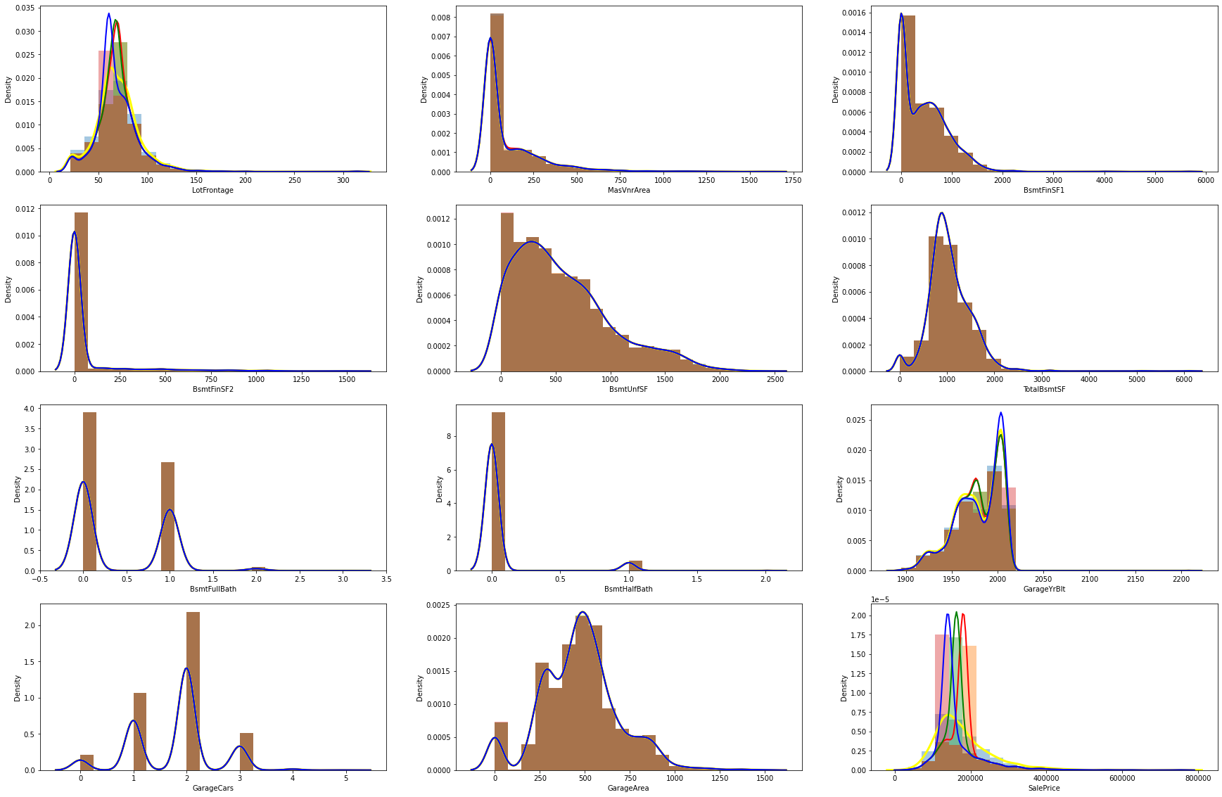
1.11 数值型特征填充前后的分布对比

# 原数值数据数据（有数据缺失的列）与使用均值、众数和中位数填充后的数据分布对比
null_numerical_features = [col for col in datas.columns if datas[col].isnull().sum()>0 and col not in non_numerical_features]
plt.figure(figsize=(30, 20))

for i, var in enumerate(null_numerical_features):
    plt.subplot(4,3,i+1)
    sns.distplot(datas[var], bins=20, kde_kws={'linewidth':3,'color':'yellow'}, label="original")
    sns.distplot(datas[var].fillna(datas[var].mean()), bins=20, kde_kws={'linewidth':2,'color':'red'}, label="mean")
    sns.distplot(datas[var].fillna(datas[var].median()), bins=20, kde_kws={'linewidth':2,'color':'green'}, label="median")
    sns.distplot(datas[var].fillna(datas[var].mode()[0]), bins=20, kde_kws={'linewidth':2,'color':'blue'}, label="mode")

1.12 时序特征分析

#------------------------------------------------------------------------------------------------------------#
# YrSold是离散型数据，YearBuilt（建房日期），YearRemodAdd（改造日期），GarageYrBlt（车库修建日期）是连续型数据
#------------------------------------------------------------------------------------------------------------#
year_feature = [col for col in datas.columns if "Yr" in col or 'Year' in col]
year_feature

['YearBuilt', 'YearRemodAdd', 'GarageYrBlt', 'YrSold']

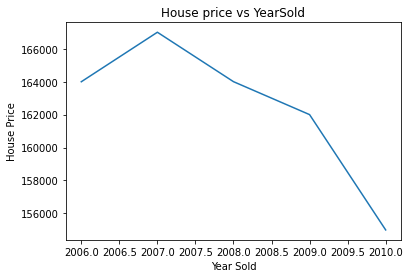
# 查看YrSold与售价的关系
datas.groupby('YrSold')['SalePrice'].median().plot()
plt.xlabel('Year Sold')
plt.ylabel('House Price')
plt.title('House price vs YearSold')

# 绘制其他三个特征与销售价格的散点对应图
for feature in year_feature:
    if feature != 'YrSold':
        hs = datas.copy()
        plt.scatter(hs[feature],hs['SalePrice'])
        plt.xlabel(feature)
        plt.ylabel('SalePrice')

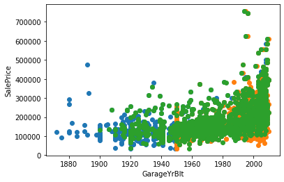
可以发现随着时间增加（即建造的时间越近），价格也逐渐增加。

1.13 用热图分析数值型特征之间的相关性

#------------------------------------------------------------------------------------------------------------#
# cmap="YlGnBu"：指定从黄绿色（正相关）到蓝绿色（负相关）的颜色渐变
# linewidths=.5：边框宽度为0.5
#------------------------------------------------------------------------------------------------------------#
plt.figure(figsize=(20,10))
numeric_features = train.select_dtypes(include=[float, int])
sns.heatmap(numeric_features.corr(), cmap="YlGnBu", linewidths=.5)

2. 数据处理

2.1 正态化 SalePrice

$n p . l o g 1 ()$ ：即计算 $l n (1 + x)$ ，使用该函数比直接使用 $n p . l o g (1 + x)$ 计算的精度要高。注意：np.log() 函数指的是计算自然对数）。
$n p . e x p m 1 ()$ ：即计算 $e^x-1$ ，使用该函数比直接计算 $e^x-1$ 的精度要高。

二者互为反函数，使用 $n p . l o g 1 ()$ 将 SalePrice 平滑化（正态化）后，最后得到的预测值需要用 $n p . e x p m 1 ()$ 进行转换。

#------------------------------------------------------------------------------------------------------------#
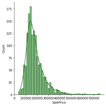
# 绘制SalePrice的特征分布
# displot：用于绘制直方图和核密度估计图
# kde：用于在直方图上叠加核密度估计曲线
# .skew()：算数据集的偏度，偏度是统计数据分布的不对称性的度量
#------------------------------------------------------------------------------------------------------------#
sns.displot(datas['SalePrice'], color='g', bins=50, kde=True)
print("SalePrice的偏度：{:.2f}".format(datas['SalePrice'].skew()))

SalePrice的偏度：1.88

在这里插入图片描述

#------------------------------------------------------------------------------------------------------------#
# 使用 np.log1() 将其平滑化（正态化）
# 偏度为1.88，SalePrice 的数据分布显著偏离正态，正常的数据应该是接近于正态分布的
#------------------------------------------------------------------------------------------------------------#
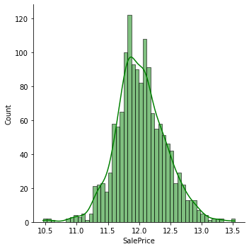
datas['SalePrice'] = np.log1p(datas['SalePrice'])
sns.displot(datas['SalePrice'], color='g', bins=50, kde=True)
print("正态化后 SalePrice 的偏度：{:.2f}".format(datas['SalePrice'].skew()))

正态化后 SalePrice 的偏度：0.12

在这里插入图片描述

2.2 时序特征处理

将时序特征离散化（用 YrSold 减去 YearBuilt、YearRemodAdd和GarageYrBlt 的时间），YrSold本身离散不用管。时序特征中 GarageYrBlt 数据有缺失，用中位数补足。

for feature in ['YearBuilt','YearRemodAdd','GarageYrBlt']:
    datas[feature]=datas['YrSold']-datas[feature]
datas['GarageYrBlt'].fillna(datas['GarageYrBlt'].median(), inplace = True)

2.3 特征融合

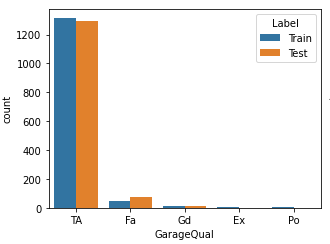
从非数值型特征的分布直方图中可以发现 GarageQual 特征的 Ex 和 Po 占比非常小（如下图），所以将这两个特征值统称为 other（其他列暂不使用，还不知道效果如何）。
在这里插入图片描述

# mask是一个布尔索引数组，长度与列 cGarageQual 的长度相同
# datas['GarageQual'][mask]：选择列 GarageQual 中所有 mask 为 True 的元素，
mask = datas['GarageQual'].isin(['Ex', 'Po'])
datas['GarageQual'][mask] = 'Other'

2.4 填充特征值

缺失最多的特征 PoolQC（泳池质量）并不代表数据缺失，而是没有泳池，因此不能简单地直接删除该列，这里用None替换掉Nan。

datas['PoolQC'].fillna("None", inplace=True)

排查数据缺失列，如果是数值型特征则根据数据 [1.11 数值型特征填充前后的分布对比] 选择中位数、众数还是平均数填充（多数情况下离散型用众数或中位数，连续型用中位数或平均数）。
如果是非数值型数据分两种情况：

缺失较多，使用 None 填充（新加一个类）
缺失较少，使用众数（最大类别）填充

# -------------------------------------------------非数值型数据----------------------------------------------#
datas['MiscFeature'].fillna('None', inplace=True)
datas['Alley'].fillna('None', inplace=True)
datas['Fence'].fillna('None', inplace=True)
datas['MasVnrType'].fillna('None', inplace=True)
datas['FireplaceQu'].fillna('None', inplace=True)
datas['GarageQual'].fillna('None', inplace=True)
datas['GarageCond'].fillna('None', inplace=True)
datas['GarageFinish'].fillna('None', inplace=True)
datas['GarageType'].fillna('None', inplace=True)
datas['BsmtCond'].fillna('None', inplace=True)
datas['BsmtExposure'].fillna('None', inplace=True)
datas['BsmtQual'].fillna('None', inplace=True)
datas['BsmtFinType1'].fillna('None', inplace=True)
datas['BsmtFinType2'].fillna('None', inplace=True)

# mode()[0]：计算该列的众数并取第一个值
datas['MSZoning'].fillna(datas['MSZoning'].mode()[0], inplace=True)
datas['Utilities'].fillna(datas['Utilities'].mode()[0], inplace=True)
datas['Functional'].fillna(datas['Functional'].mode()[0], inplace=True)
datas['Electrical'].fillna(datas['Electrical'].mode()[0], inplace=True)
datas['Exterior2nd'].fillna(datas['Exterior2nd'].mode()[0], inplace=True)
datas['Exterior1st'].fillna(datas['Exterior1st'].mode()[0], inplace=True)
datas['SaleType'].fillna(datas['SaleType'].mode()[0], inplace=True)
datas['KitchenQual'].fillna(datas['KitchenQual'].mode()[0], inplace=True)

#--------------------------------------------------数值型数据------------------------------------------------#
datas['MasVnrArea'].fillna(datas['MasVnrArea'].mean(), inplace = True)
datas['LotFrontage'].fillna(datas['LotFrontage'].mean(), inplace = True)
datas['BsmtFullBath'].fillna(datas['BsmtFullBath'].median(), inplace = True)
datas['BsmtHalfBath'].fillna(datas['BsmtHalfBath'].median(), inplace = True)
datas['BsmtFinSF1'].fillna(datas['BsmtFinSF1'].median(), inplace = True)
datas['GarageCars'].fillna(datas['GarageCars'].mean(), inplace = True)
datas['GarageArea'].fillna(datas['GarageArea'].mean(), inplace = True)
datas['TotalBsmtSF'].fillna(datas['TotalBsmtSF'].mean(), inplace = True)
datas['BsmtUnfSF'].fillna(datas['BsmtUnfSF'].mean(), inplace = True)
datas['BsmtFinSF2'].fillna(datas['BsmtFinSF2'].median(), inplace = True)

数据填充完之后确认一下是否还有遗漏的数据

datas.isnull().sum().sort_values(ascending = False).head(10)

SalePrice       1459
MSZoning           0
GarageYrBlt        0
GarageType         0
FireplaceQu        0
Fireplaces         0
Functional         0
TotRmsAbvGrd       0
KitchenQual        0
KitchenAbvGr       0
dtype: int64

2.5 连续性数据正态化

数据填充完毕后，重新挑选出连续型数值特征，观察其分布情况。

numerical_features = [col for col in datas.columns if datas[col].dtypes != 'O']
discrete_features = [col for col in numerical_features if len(datas[col].unique()) < 25 and col not in ['Id']]
continuous_features = [feature for feature in numerical_features if feature not in discrete_features+['Id']]
fig,axes = plt.subplots(nrows = 4, ncols = 6, figsize=(30,15), sharex=False)
for i, feature in enumerate(continuous_features):
    sns.histplot(data=datas, x=feature, hue='Label',ax=axes[i%4,i//4])

在这里插入图片描述
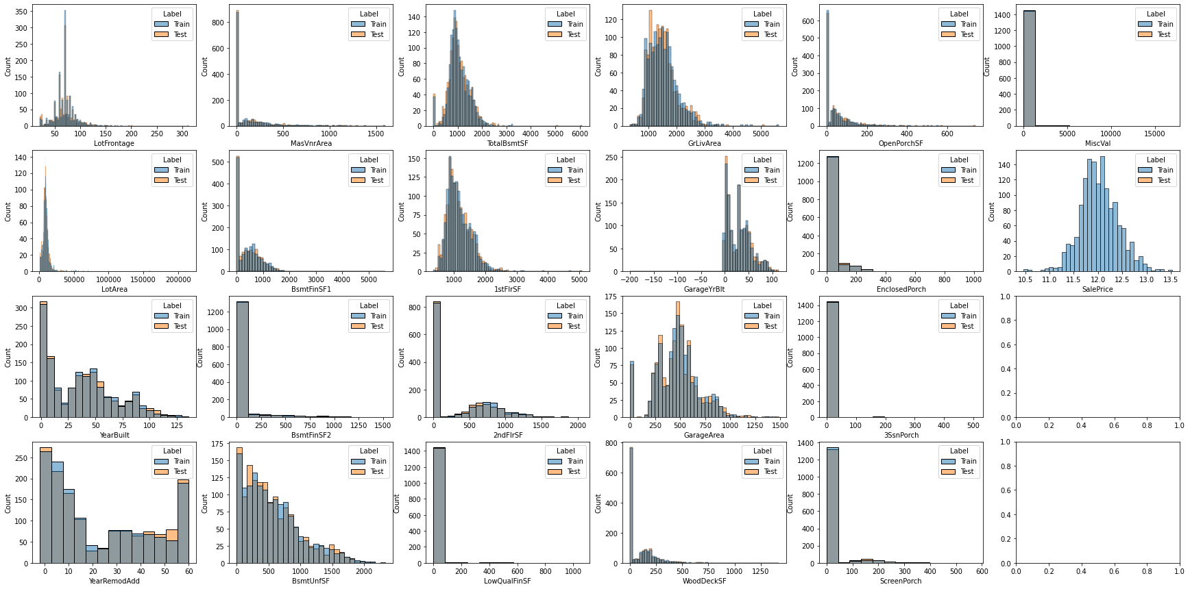
通过直方图可以直观地看出数值的分布是否符合正态分布，再分别计算偏度，通过偏度查看数据的偏离情况。

# 计算偏度
skewed_features = datas[continuous_features].apply(lambda x:x.skew()).sort_values(ascending=False)
print(skewed_features)

MiscVal          21.958480
LotArea          12.829025
LowQualFinSF     12.094977
3SsnPorch        11.381914
BsmtFinSF2        4.148275
EnclosedPorch     4.005950
ScreenPorch       3.948723
MasVnrArea        2.612892
OpenPorchSF       2.536417
WoodDeckSF        1.843380
LotFrontage       1.646420
1stFlrSF          1.470360
BsmtFinSF1        1.426111
GrLivArea         1.270010
TotalBsmtSF       1.163082
BsmtUnfSF         0.919981
2ndFlrSF          0.862118
YearBuilt         0.598917
YearRemodAdd      0.450458
GarageYrBlt       0.392261
GarageArea        0.241342
SalePrice         0.121347
dtype: float64

这里将偏度大于 1.5 的特征进行正态化，值设得太大的话正态化之后会导致原本0-1之间的特征的偏度过于小（-4左右）而出现左偏斜（即数据集中有较多较小的值）。

# 如果偏度的绝对值大于1.5，则用np.log1p进行处理【注：并不保证处理后偏度就会小于1.5，只能是使数据尽量符合正态分布】
# 需要正则化的特征列
log_list=[]
for feature, skew_value in skewed_features.items():
    if skew_value > 1.5:
        log_list.append(feature)
log_list

# 正则化
for i in log_list:
    datas[i] = np.log1p(datas[i])
  
# 检查正则化情况
skewed_features = datas[continuous_features].apply(lambda x:x.skew()).sort_values(ascending=False)
print(skewed_features)

3SsnPorch        8.829794
LowQualFinSF     8.562091
MiscVal          5.216665
ScreenPorch      2.947420
BsmtFinSF2       2.463749
EnclosedPorch    1.962089
1stFlrSF         1.470360
BsmtFinSF1       1.426111
GrLivArea        1.270010
TotalBsmtSF      1.163082
BsmtUnfSF        0.919981
2ndFlrSF         0.862118
YearBuilt        0.598917
MasVnrArea       0.504832
YearRemodAdd     0.450458
GarageYrBlt      0.392261
GarageArea       0.241342
WoodDeckSF       0.158114
SalePrice        0.121347
OpenPorchSF     -0.041819
LotArea         -0.505010
LotFrontage     -1.019985
dtype: float64

由结果可知，3SsnPorch、LowQualFinSF 和 MiscVal 的偏度还是太大（正偏度值大于2通常被认为是严重的右偏斜），但此时不宜再对这三个特征再次进行正态化，否则可能会导致数据失真。

2.5 编码数据集后切分数据集

# 删除Label列后对数据集进行独热（One-hot）编码
datas.drop('Label', axis=1, inplace=True)
datas = pd.get_dummies(datas, dtype=int)
# 切分训练集和测试集
new_train= datas.iloc[:len(train), :]
new_test = datas.iloc[len(train):, :]
X_train = new_train.drop('SalePrice', axis=1)
Y_train = new_train['SalePrice']
X_test = new_test.drop('SalePrice', axis=1)

3. 模型搭建

3.1 模型搭建与超参数调整

import optuna
from sklearn.linear_model import Ridge
from xgboost import XGBRegressor
from sklearn.ensemble import GradientBoostingRegressor
from sklearn.model_selection import cross_val_score

"""
定义超参数优化函数
Params：
    objective：待优化的评估函数
Returns:
    params：最佳超参数组合
"""
def tune(objective):
    # 创建了一个 Optuna 的 Study 对象，用于管理一次超参数优化的过程
    # direction='maximize' 表示优化的目标是最大化目标函数的返回值（返回值是负的均方根误差）
    study = optuna.create_study(direction='maximize')
    
    # 使用 study 对象的 optimize 方法来执行优化过程
    # n_trials=100：指定了进行优化的试验次数
    study.optimize(objective, n_trials=10)
    
    params = study.best_params
    # 获取经过优化后的最佳得分（（目标函数的返回值））
    best_score = study.best_value
    print(f"Best score: {-best_score} \nOptimized parameters: {params}")
    return params

"""
Ridge回归
Params：
    trial：是由 Optuna 库提供的对象，用于在超参数优化过程中管理参数的提议和跟踪
Returns:
    score：交叉验证评分
"""
def ridge_objective(trial):
    # 0.1 是超参数的下界，20 是超参数的上界。Optuna 会在指定的范围内为超参数 alpha 提出一个值
    _alpha = trial.suggest_float("alpha",0.1,20)
    ridge = Ridge(alpha=_alpha, random_state=1)
    score = cross_val_score(ridge,X_train,Y_train, cv=10, scoring="neg_root_mean_squared_error").mean()
    return score

"""
梯度增强树回归
Params：
    trial：是由 Optuna 库提供的对象，用于在超参数优化过程中管理参数的提议和跟踪
Returns:
    score：交叉验证评分
"""
def gbr_objective(trial):
    _n_estimators = trial.suggest_int("n_estimators", 50, 2000)
    _learning_rate = trial.suggest_float("learning_rate", 0.01, 1)
    _max_depth = trial.suggest_int("max_depth", 1, 20)
#     _min_samp_split = trial.suggest_int("min_samples_split", 2, 20)
#     _min_samples_leaf = trial.suggest_int("min_samples_leaf", 2, 20)
#     _max_features = trial.suggest_int("max_features", 10, 50)

    gbr = GradientBoostingRegressor(
        n_estimators=_n_estimators,
        learning_rate=_learning_rate,
        max_depth=_max_depth, 
#         max_features=_max_features,
#         min_samples_leaf=_min_samples_leaf,
#         min_samples_split=_min_samp_split,
        
        random_state=1,
    )

    score = cross_val_score(gbr, X_train,Y_train, cv=10, scoring="neg_root_mean_squared_error").mean()
    return score

"""
XGBoost回归模型
Params：
    trial：是由 Optuna 库提供的对象，用于在超参数优化过程中管理参数的提议和跟踪
Returns:
    score：交叉验证评分
"""
def xgb_objective(trial):
    _n_estimators = trial.suggest_int("n_estimators", 50, 2000)
    _max_depth = trial.suggest_int("max_depth", 1, 20)
    _learning_rate = trial.suggest_float("learning_rate", 0.01, 1)
#     _gamma = trial.suggest_float("gamma", 0.01, 1)
#     _min_child_weight = trial.suggest_float("min_child_weight", 0.1, 10)
#     _subsample = trial.suggest_float('subsample', 0.01, 1)
#     _reg_alpha = trial.suggest_float('reg_alpha', 0.01, 10)
#     _reg_lambda = trial.suggest_float('reg_lambda', 0.01, 10)

    xgboost = XGBRegressor(
        n_estimators=_n_estimators,
        max_depth=_max_depth, 
        learning_rate=_learning_rate,
#         gamma=_gamma,
#         min_child_weight=_min_child_weight,
#         subsample=_subsample,
#         reg_alpha=_reg_alpha,
#         reg_lambda=_reg_lambda,
#         random_state=1,
    )
    score = cross_val_score(xgboost, X_train, Y_train, cv=10, scoring="neg_root_mean_squared_error").mean()
    return score

寻找最佳参数，运行下面代码很耗时，可适当减少不重要参数的调优。本地调优后官网提交时不用再次运行，直接用本地运行的最佳参数即可。

# 设置日志级别为 WARNING，减少输出信息的数量
# optuna.logging.set_verbosity(optuna.logging.WARNING)

ridge_params = tune(ridge_objective)
# Best score: 0.13482720346041538 
# Optimized parameters: {'alpha': 14.933121817345844}
# ridge_params = {'alpha': 14.933121817345844}
    
gbr_params = tune(gbr_objective)
# Best score: 0.1388996815131788 
# Optimized parameters: {'n_estimators': 928, 'learning_rate': 0.24282934638611978, 'max_depth': 7}
# gbr_params = {'n_estimators': 928, 'learning_rate': 0.24282934638611978, 'max_depth': 7}

xbg_params = tune(xgb_objective)
# Best score: 0.12403838351336531 
# Optimized parameters: {'n_estimators': 1713, 'max_depth': 3, 'learning_rate': 0.030462678052628034}
# xbg_params = {'n_estimators': 1713, 'max_depth': 3, 'learning_rate': 0.030462678052628034}
              
# **：用于将键值对作为关键字参数传递给函数
ridge = Ridge(**ridge_params, random_state=1)
gbr = GradientBoostingRegressor(**gbr_params, random_state=1)
xgboost = XGBRegressor(**xbg_params, random_state=1)

3.2 模型交叉验证

ridge_score = np.sqrt(-cross_val_score(ridge, X_train, Y_train, cv=10, scoring='neg_mean_squared_error')) 
gbr_score = np.sqrt(-cross_val_score(gbr, X_train, Y_train, cv=10, scoring='neg_mean_squared_error')) 
xgboost_score = np.sqrt(-cross_val_score(xgboost, X_train, Y_train, cv=10, scoring='neg_mean_squared_error')) 
print(f"ridge_score: {np.mean(ridge_score)}")
print(f"gbr_score: {np.mean(gbr_score)}")
print(f"xgboost_score: {np.mean(xgboost_score)}")

ridge_score: 0.13482720346041538
gbr_score: 0.1388996815131788
xgboost_score: 0.12403838351336531

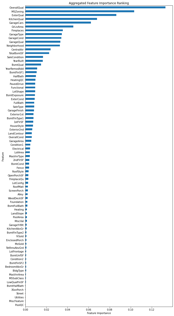
3.3 特征重要性分析

xgboost.fit(X_train, Y_train)
# 删除 "SalePrice" 方便分析特征重要性
imp_datas = datas.drop("SalePrice", axis=1)

# 获取特征重要性
importance = xgboost.feature_importances_

# 创建特征名称与重要性映射，用于合并独热编码之后的特征
feature_importance = pd.Series(importance, index=imp_datas.columns)

# 提取独热编码的特征名
original_feature_names = [col.split('_')[0] for col in imp_datas.columns]

# 聚合特征重要性
aggregated_importance = feature_importance.groupby(original_feature_names).sum()

plt.figure(figsize=(10, 18))

# kind='barh'：指定了绘图类型为水平条形图
# sort_values()本身是由小到大的排序，但使用 .plot(kind='barh') 时，水平条形图的 y 轴将显示由高到低的顺序
aggregated_importance.sort_values().plot(kind='barh')
plt.xlabel("Feature Importance")
plt.ylabel('Feature')
plt.title("Aggregated Feature Importance Ranking")
# 调整图表布局，使其更紧凑
plt.tight_layout()

在这里插入图片描述

3.4 数值预测

选择最佳模型xgboost预测售价。

xgboost.fit(X_train, Y_train)
predictions = np.expm1(xgboost.predict(X_test))
submission = pd.DataFrame({'Id': Id,'SalePrice': predictions})
# submission.to_csv('/kaggle/working/submission.csv', index=False)
print('Submission file created!')